Deep Q-Networks (DQN)
In the previous posts, we looked at small environments like the grid world. In these environments it is easy to create a table that contains an action for each state. But what happens if the state space is huge, like e.g. in the game Go. Then this tabular approach is not possible anymore.
In this post, we discuss how we can extend Q-Learning to huge state spaces by using function approximation. We will use a Neural Network for this. The reader is assumed to have a basic knowledge of it. Some short introduction can be found in wikipedia: Artificial Neural Network.
Function Approximation
Assume we have a huge state space, like in the board game of Go. On a game board with a size of 19 x 19 there are more than \(10^{170}\) legal positions. It’s not feasible to store this in a tabular form on a computer due to the shortage of memory.
Besides the memory problem, there is also a problem with filling the table. To add an entry, the corresponding state has to be visited. That’s often infeasible as well.
How can we solve these issues? The solution is to use function approximation for the complex non-linear function Q(s,a).
This obviously saves the memory issues, as we just need to store the function instead of the whole table.
It also solves the visiting of each state. This means that we can even estimate Q(s,a) values for states that we haven’t estimated so far. The main assumption is that states that are close to each other result in the same action. This means visiting a state s also enables estimates for all close states.
There are multiple approaches to approximate this function. Some are described in the excellent book of Richard Sutton, which can be downloaded for free: Reinforcement Learning: An Introduction.
In the following we will focus on using a Deep Neural Network as function approximation.
Neural Network
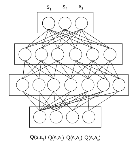
A neural network is just a collection of connected neurons (nodes). It consists of an input layer, multiple hidden layers and an output layer ( wikipedia: Artificial Neural Network).
The input layer takes the representation of the state of the environment as input. This representation can be an image, as in the case of the Atari games. But it could also be something like position, velocity, acceleration, … It’s important that this representation contains all the relevant information about the environment, as this is the data the agent uses for learning.
The output contains a q-value for each action.
An example network is shown in the figure below. It’s just a sketch, and thus actually the edges between nodes are not complete. The neural network takes the state represented by \(s_1, s_2, s_3\) as input. Assuming, that we have four discrete actions, it outputs a q-value corresponding to each possible action. We then execute the action with the highest value.
How can we train this Neural Network?
Actually, we can use a supervised learning approach. Our target (label) can be retrieved from the Bellman Equation we discussed in Temporal Difference Learning post.
\[Q(s,a) = \mathbb{E}[ r(s,a) + \gamma \mathbb{E}[Q(s',a')]]\]From this, we derived our Q-Learning formula:
\[Q(s,a) = Q(s,a) + \alpha * (r(s,a) + \gamma * \max_{a'}Q(s',a') - Q(s,a))\], where \(r(s,a) + \gamma * \max_{a'}Q(s',a') - Q(s,a)\) is the error \(\delta\).
We want to minimize the square of this error. This can be done by backpropagation.
Unfortunately, it’s not possible to directly use the data when it is coming from the environment. This means when we collected the experience (s,a,r,s’) we can’t directly update the weights of the Neural Network.
That’s a problem, and in the following we discuss why it is a problem and how to overcome it.
Experience Replay
Training a Neural Network with backpropagation uses stochastic gradient descent. This algorithm assumes that the training data is independent and identically distributed (i.i.d). Unfortunately, our training data doesn’t fulfill this assumption.
It is not independent, as the data received is coming from an agent that is following a policy. In other words, the next state and the current state are coupled by the current policy temporarily. Thus, the agent can’t learn directly from the experiences.
This problem can be addressed with a buffer. The buffer stores the data collected through many episodes. The stored experiences are (s,a,r, s’). During the learning process, a subset is sampled randomly from the buffer. This approach leads to the fulfillment of i.i.d experiences, and thus we can train our Neural Network.
A simple implementation of a buffer is a ring buffer of a fixed size. Mainly in the order of at least 100,000. This means that if the buffer is full, a newly added experience pushes out the oldest one.
The buffer in this context is called replay buffer as you replay experiences that you have recorded.
The process of sampling a subset from the replay buffer to learn from it is called experience replay.
Target Networks
We used supervised learning for training. Unfortunately, the approach is not directly supervised learning, as the target depends on the network weights. The target is
\[y_i = r_i(s,a) + \gamma \max_{a'}Q_{\phi}(s',a')\], where \(Q_{\phi}\) stands for Q being parametrized by \(\phi\). The problem is that updating the weights that \(Q_{\phi}(s,a)\) is closer to y_i can also change y_i.
That’s because \(Q_{\phi}(s,a)\) and \(Q_{\phi}(s',a')\) depend on the same weights. Thus, updating the weights leads to changing the target as well as the estimation. This can lead to an unstable learning process.
The learning process can be made more stable by using a target network. The target network is a copy of the original network and is used to estimate \(Q_{\phi}(s',a')\). The original network is updated during training. After some episodes, the learned weights are copied to the target network.
Thus, we need to update the formula to:
\[y_i = r_i(s,a) + \gamma \max_{a'}Q_{T_{\phi}}(s',a')\], where \(Q_{T_{\phi}}\) is the target network.
The additional target network stabilizes the learning process.
Problems of DQN
The algorithm we described above is called Deep Q-Learning (DQN).
It takes a representation of the state as input and outputs all the state action values. But what happens if the action space is continuous. Imagine choosing the intensity of an action instead of only deciding which action to execute. How could a DQN handles this case?
One way would be to discretize the action space. But how fine granular do you want to discretize the space.
Furthermore, DQN has problems with high dimensional action spaces. Imagine the robot Atlas from Boston Dynamics. It has 28 degrees of freedom. If we discretize the action for each degree into 10 possible ways, we would have \(10^{28}\) output neurons. Finding the maximum would be an optimization issue on its own.
Many of these issues come from the fact that we estimate the state action values and then select the action with the highest value. But why do we do this extra step. Can’t we directly estimate the action instead of first calculating the q-values?
The good thing is that it’s possible to skip the q-value calculation and go directly to the action. This will be discussed in detail in one of the next posts.
Summary
We discussed the problems of Q-Learning with a huge state space and discrete action space. Then we solved the problems by using function approximation instead of a tabular approach. We used a Neural Network for function approximation, which lead us to the famous DQN algorithm.
More information can be found in the papers from Deepmind.
- Playing Atari with Deep Reinforcement Learning
- Human-level control through deep reinforcement learning
Nevertheless, we discovered that DQN has issues with continuous and high dimensional action spaces. We will come up with a solution for this issue in one of the next posts. The solution we will look at will be a policy gradient algorithm.