Reinforcement Learning Basics

This post gives an introduction to reinforcement learning (RL). It describes all components that are part of it and how they are connected. The goal is to get an intuitive understanding of why it is so amazing. After reading it, you should know which kind of problem reinforcement learning is trying to solve.

Reinforcement Learning is a subfield of machine learning and focuses on learning by trial and error. This is very cool, isn’t it? Just imagine a chess engine that learns to play chess on its own, without any expert knowledge (except the allowed moves of the single pieces). The chess engine just plays a game and in the end receives a reward (+1 for winning, 0 for draw and -1 for losing). Only by this feedback, the engine is able to learn to play chess extremely well. That’s fascinating.

Reinforcement learning gets a lot of popularity since 2016 when the strongest Go Player in the world (Lee Sedol) was beaten by AlphaGo in the game Go. AlphaGo is an algorithm that was developed by Google Deepmind. This was a huge milestone, as Go was not expected to be beaten by an algorithm in the near feature. This assumption was based on the fact that the game has a very huge amount of possible states. On a board size of 19 x 19 there are more than \(10^{170}\) legal positions.

Key concepts

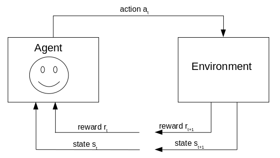
The agent is in a state s_t and interacts with the environment by executing action a_t. By this interaction, the environment changes into a new state s_t+1. At the same time, the agent receives a reward r_t+1 that contains information on how good this action was. This feedback is used by the agent to learn which action is good in which state. The agent chooses its actions to maximize the rewards he can collect.

At first, we will look at the terminology and afterwards at a concrete example.

Agent

The agent interacts with the environment by executing actions. Its goal is to receive as much reward as possible.

Environment, State and Observation Space

The environment is completely described by the state s. In contrast to that, an observation o is just a partial description of the state.

Imagine a vacuum cleaner (agent) that has the task to clean the rooms of a house. The state s contains information about all rooms in the house. The vacuum cleaner itself only has partial information about the room it is. This is due to the limiting range of the sensor it is equipped with. It only can detect its surrounding.

The reinforcement learning literature doesn’t really differentiate between these two. They often talk about states even though the correct term would be observation. Thus, I also use the more common wording of sates, even though sometimes the correct wording would be observation. The state space S consists of the set of valid states and the observation Space O of the set of valid observations.

Discrete and Continuous Action Spaces

The action space A contains all the actions a that an agent can execute. These are highly dependent on the environment.

This makes sense. If you play the game monopoly you can e.g. buy a property, construct a hotel or throw the dices. In contrast to that, if you play soccer you can e.g. pass the ball, dribble or shoot.

The action space could either be discrete or continuous. Discrete means to have a finite amount of actions. Imagine an easy computer game where you can only go left or right. In contrast to that, continuous action spaces have an infinite amount of possible actions. Imagine soccer, where you not only have the shoot action, but the possibility to vary the intensity of the shoot as well.

Return and Reward

The reward is a very important part of reinforcement learning. This actually tells the agent which behaviour is good (high reward) or which is bad (low reward). Thus, it defines what behaviour the agent learns at the end. We will look at some examples of how the reward influences the behaviour of the agent in a later section.

The reward is what the agent gets from the environment after he executes an action a_t in state s_t and ends up in a new state s_t+1. This means that the reward r can be seen as a function \(R : S \times A \times S \to \mathbb{R}\).

The goal of the agent is to maximize the cumulative rewards during some trajectory \(\tau\). A trajectory is simply a sequence of states and actions. \(\tau = (s_t, a_t,s_{t+1},a_{t+1},...)\). The cumulative reward is called return R. This means the agent wants to maximize the return until the final time stamp T.

\[R(\tau) = \sum_{t=0}^T r_{t}\]

How is this final time step defined? In games, the final time step is obviously the winning/draw/losing state. Here the trajectory \(\tau\) has a defined length and is called an episode. The task is called episodic.

But this is very different for other tasks that are continuing over a long period of time. This is e.g. the case in controlling the heat of a room. The trajectory is infinite, and we call it a continuing task.

In a continuing task (\(T = \infty\)), the return is not converging to a finite value. To prevent this, we add a discount factor \(\gamma\in[0,1)\). This factor guarantees a convergence.

\[R(\tau) = \sum_{t=0}^{\infty} \gamma^{t} r_{t}\]

The discount factor is also useful for episodic tasks, as it encodes that a reward now is more worth than in the future. This forces the agent to achieve its goal as fast as possible, and that’s what we actually want.

Policy

The policy \(\pi\) is the brain of the agent and selects the action it should take in each state. It is a mapping from states to a probability distribution over the actions. The goal of reinforcement learning is to find an optimal policy \(\pi^*\).

\[a_{t} \sim \pi(s_{t})\]

The policy is called deterministic if in each state, one action has probability 1 and thus the others have 0. Intuitively, this means that you exactly know which action the agent picks in state s.

Otherwise, the policy is called stochastic. In this case, you don’t know exactly which action is picked. You just know the probability distribution. An example for state \(s_{1}\) could be \(\pi(a_{1}|s_{1})= 0.3\), \(\pi(a_{2}|s_{1})= 0.5\) and \(\pi(a_{3}|s_{1})= 0.2\). Where \(\pi(a_{1}|s_{1})\) means the probability of selecting action \(a_1\) in state \(s_1\).

State Value Function and Action Value Function

A state value function \(V: S \to \mathbb{R}\) maps states to a value. This value represents the expected return the agent gets if he starts in a state and then acts according to its policy.

\[V^{\pi}(s) = \mathbb{E}_{\pi}[R_t(\tau) | S_t=s] = \mathbb{E}_{\pi} [\sum_{k=0}^{\infty} \gamma^k r_{t+1+k}]\]

How can this value help us? In the end we are interested in a policy \(\pi\) and that is a mapping from state to action.

One approach is to evaluate for each possible action in state s what the reward belongs to this action and what is the expected return of the state s’ we end up by this action.

\[a = \operatorname*{arg\max}_{a \in A}\mathbb{E}_{\pi}[R_a(s,s') + V(s')]\]

This is a valid solution in a Markov Decision Process, as there we know the state transition function, meaning that we know in which state S’ we end if we execute action a in state s. In reinforcement learning, we unfortunately don’t know this.

Thus, instead of storing only the expected return for a state, we store the expected return for each action we can do in that state. This function is called action value function.

\[Q^{\pi}(s, a)= \mathbb{E}_{\pi}[R_t(\tau) | S_t=s, A_t=a]\]

Having the q-values stored for each state, we can easily choose the action that returns the highest expected return.

\[Q(s, a)=\operatorname*{arg\max}_{a \in A}Q(s,a)\]

Optimal Value Function

We already talked a few times about the optimal value function and the improved or optimal policy. We intuitively understand what is meant by that. But we missed a formal definition so far. A policy \(\pi\) is better than a policy \(\pi'\):

\[\pi \geq \pi' \text { if and only if } V^{\pi}(s) \geq V^{\pi'}(s), \forall s \in S\]

The optimal value function is defined as:

\[V^*(s) = \operatorname*{max}_{\pi} V^{\pi}(s)\]

Analogously, we can define the optimal action value function:

\[Q^*(s,a) = \operatorname*{max}_{\pi} Q^{\pi}(s,a)\]

The Goal of Reinforcement Learning

In the beginning, we said that the goal of the agent is to maximize the expected return \(J\). Let’s define this in a more formal way.

\[J(\pi) = \mathbb{E}_{\tau \sim \pi}[R(\tau)] =\sum_{\tau} P(\tau|\pi)R(\tau)\]

\(P(\tau|\pi)\) describes how probable it is to see the trajectory \(T\) under the policy \(\pi\). Thus, we weight the reward of each trajectory by the probability of seeing it under this policy.

Markov Decision Process (MDP)

All the concepts described above most probably already sound familiar to you. That’s because it’s describing a Markov Decision Process. You can have a look at it in e.g. wikipedia.

But if reinforcement learning can be modelled as a MDP, what is then the problem? Can’t we just solve it with dynamic programming as usual? The difficulty is that we don’t know the dynamics of the environment and thus can’t easily solve it. This means that the agent does not a priori knows what happens if he executes an action in a state.

The agent needs to discover the dynamics of the environment by trial and error. Trial and error means to execute different actions in different states and see which rewards he receives.

Example

This example illustrates the concepts described earlier. We will not discuss how the agent learns. That will be part of a follow-up post. The main focus will be on getting a visual understanding of the reinforcement learning problem statement.

Imagine we have a 4x4 grid world and the goal of the agent is to find the star. See in the image below. This environment has 16 states. The start position of the agent is (0,0) and the goal state is (3,3). The task is episodic, which means that if the agent reaches the goal state, the episode terminates. Now everything is set back, and the agents starts again.

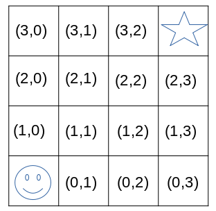
We define that the agent has 4 different actions (up, down, left or right). This means that if the agent executes action up in state (0,0) he will end up in state (1,0). If he evaluates an action that he can’t do as there is a border, he will stay in the same state. This means that action left in state(1,0) will lead to state(1,0).

In the preceding paragraph, we have described the action and state space. One important thing is missing. We need to define a reward function such that the agent quickly moves to the goal position (star). Let’s keep it simple and say that we use a discounted reward function with \(\gamma = 0.9\) and that reaching the goal state gives a reward of +1, while all other rewards are 0.

Finally, we have everything ready to start with reinforcement learning. Let’s dive into this interesting part.

In the beginning, the agent doesn’t know anything about the environment. The only thing he can do is to make random actions. Thus, he goes left, right, up, up, down, …. As the agent is always getting a reward of 0 he can’t learn anything. This goes on until the agent reaches the star. He receives a reward of +1, which we have specified for reaching this state.

This is the first time the agent gets valuable feedback. Assuming he reached the goal state from state (3,2) with action right, he now knows that this action was a good one to make. But maybe there is even a better action. To learn more about the environment, the agent now starts again from state (0,0).

This goes on for a while, and the agent understands more and more which action in which state is good. In other words, the policy of the agents improves, which leads to a higher expected return.

After running for multiple episodes, the agent has a good policy and knows how to reach the goal state. The agent knows which action to chose in which state. But he never knows if there is a better action to select in a state. This is called the exploration vs. exploitation dilemma. A paper about this can be found here: Exploration vs. Exploitation

Let’s illustrate this dilemma. Imagine you are new in a town and want to find a good pizzeria. At the beginning, you will try a few and then decide on a favourite on, which you like more than the others. But possibly there is even a better one in town. But you don’t know. Thus, each time you go for a pizza, you either exploit your knowledge, and you go to your favourite one. Or you try to find a better one, and thus you try a new one (exploration).

Influence of the Reward on the Behaviour of the Agent

The chosen reward function is very important and often not so easy as in this toy example. Let’s see how it influences the behaviour of the agent.

The easiest reward function for the grid world is to give the robot +1 if he reaches the goal state, and 0 in all other cases. The robot learns to reach the goal. Is it the fastest way he learns?

No, he doesn’t. At least if we set \(\gamma\) to 1. There is no difference in reward for the agent if he reaches the goal after time step t₁ or t_x. Thus, normally future rewards are discounted by \(\gamma\) as shown above. This forces the agent to learn the fastest route, as rewards at an earlier time step are worth more than at a later one.

Another way to reach the goal faster, with \(\gamma=1\), would be to reward the agent with +1 if he reaches the goal. And a reward of -0.1 for each time step. To maximize the expected return the agent would try to go to the goal as fast as possible.

What would happen if we set the reward for each time step to a value > 0 and the reward for the goal state to +1. What strategy would he learn?

Actually, in this case the agent would learn to never reach the goal state. That’s because he gets a positive reward for each step. If the agent reaches the goal state, this reward would stop as the episode is finished. Thus, he tries to avoid it.

Summary

As you seen above, the only thing to make an agent learn what you want is to specify a reward function. Just think about it again. You just need to specify a reward function. Okay, this is a bit simplified, as finding a good is often still complex.

But you don’t need to come up with very domain specific algorithms that are hardcoded into the agent. For the simple case as seen above, it would be easy to implement an algorithm. But imagine a more complex environment like for example autonomous driving. Here exist so many scenarios that it is infeasible to specify an action for each state. The same is true for the games Chess and Go. In these cases, reinforcement learning is a perfect algorithm to choose.

In these use cases reinforcement learning is a perfect solution and achieves excellent results as can be seen by AlphaGo.