Monte Carlo Methods

In the post about the reinforcement learning basics we looked at the key concepts of reinforcement learning and what problem we actually want to solve. Now we want to address how this problem can be solved. There are multiple methods and in this post we want to have a closer look at Monte Carlo Methods.

Finally, we are ready to solve our first reinforcement learning problem. This will be amazing. At first we need to specify the environment we want to solve.

The Grid World

Welcome back to our 4x4 grid world we already visited in the last post. Lets’s quickly recap the setting.

Imagine we have a 4x4 grid world and the goal of the agent is to find the star. See in the image below. This environment has 16 states. The start position of the agent is (0,0) and the goal state is (3,3). The task is episodic, which means that if the agent reaches the goal state, the episode terminates. Now everything is set back, and the agents starts again.

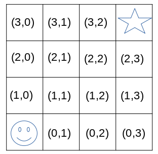
We define that the agent has 4 different actions (up, down, left or right). This means that if the agent executes action up in state (0,0) he will end up in state (1,0). If he evaluates an action that he can’t do as there is a border, he will stay in the same state. This means that action left in state(1,0) will lead to state (1,0).

Solving the Grid World

The goal of the agent is to reach the start, which is in the top right corner. We define the reward function as +1 for reaching the star and 0 otherwise. The discount factor \(\gamma = 0.9\). The influence of the reward function on the behaviour of the agent was already discussed in the reinforcement learning basics post.

The agent has no knowledge about the dynamics of the environment and thus moves according to its starting policy \(\pi_{0}\), which normally results in random behaviour. The agent chooses actions according to this policy and tries to learn a better one. This means to achieve a higher expected return.

Let’s assume this is the first trajectory of the agent:

\[\tau^{\pi_0}=((0,0),up,0,(1,0),right,0,(1,1),...,(3,2),right,1,(3,3))\]

The trajectory is represented by the blue arrows in the image below.

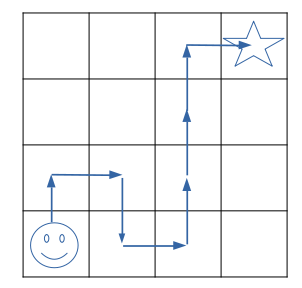
What has the agent learned now? He learned that action right in state (3,2) is good, as he got a reward of +1. This is very obvious. But what about all the other states that are part of this trajectory. After the first trajectory, the agent has the following information.

\[Q^{\pi_0}((3,2),right) = 1\] \[Q^{\pi_0}((2,2), up) = 0 + \gamma * 1\] \[Q^{\pi_0}((1,2), up) = 0 + \gamma * 0 + \gamma^2 * 1\] \[Q^{\pi_0}((0,2), up) = 0 + \gamma * 0 + \gamma^2 * 0 + \gamma^3 * 1\] \[Q^{\pi_0}((0,1), right) = 0 + \gamma * 0 + ... + \gamma^4 * 1\] \[Q^{\pi_0}((1,1), down) = 0 + \gamma * 0 + ... + \gamma^5 * 1\] \[Q^{\pi_0}((1,0), right) = 0 + \gamma * 0 + ... + \gamma^6 * 1\] \[Q^{\pi_0}((0,0), up) = 0 + \gamma * 0 + ... + \gamma^7 * 1\]

The agent learned some information about the environment. He learned one path to reach the goal state. If we choose as policy to always use the maximum q-value in each state, then we would always take the same path. Meaning, the agent exploits it’s knowledge about a path that leads to the goal. Unfortunately, this learned path does not need to be the optimal one.

Looking at our first trajectory, we know it’s not perfect. It would be better if the agent in state (1,1) takes action right instead of going down. But the agent doesn’t know that.

To avoid this exploitation-exploration dilemma as discussed in a previous post we need some randomness in mapping states to action. A simple and common approach is to use an \(\epsilon- greedy\) approach, where \(epsilon \in [0,1]\). This means, that we take the best action with a probability of \(1-\epsilon\) and with a probability of \(\epsilon\) we take a random action. This, supports the agent to continue exploration during training.

After the q-values are updated, the agent now has a new policy \(\pi_1\) Let’s assume the second trajectory of the agent looks like shown in the image below.

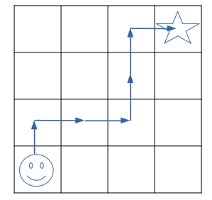
The agent now has this information, additional to the one from the first trajectory.

\[Q^{\pi_1}((3,2),right) = 1\] \[Q^{\pi_1}((2,2), up) = 0 + \gamma * 1\] \[Q^{\pi_1}((1,2), up) = 0 + \gamma * 0 + \gamma^2 * 1\] \[Q^{\pi_1}((1,1), right) = 0 + \gamma * 0 + \gamma^2 * 0 + \gamma^3 * 1\] \[Q^{\pi_1}((1,0), right) = 0 + \gamma * 0 + ... + \gamma^4 * 1\] \[Q^{\pi_1}((0,0), up) = 0 + \gamma * 0 + ... + \gamma^5 * 1\]

The agent now learned that in state (1,1) the action right is better than action down as Q((1,1), right) > Q((1,1), down). But it still doesn’t know if there still exists a better trajectory.

Now, the agent would sample a third trajectory, then a fourth and so on.

During the training, the agent visits the same state action pairs Q(s,a) multiple times. This could potentially lead each time to a different return, as it depends on the policy that is used for this trajectory. We will average all this values. By the law of large numbers, the averages of these estimates converges to the expected return.

This approach leads finally to the optimal state action value, and thus our agent can solve the grid world in a perfect way.

This kind of sample based method is called Monte Carlo Methods, and we will formalize a pseudocode algorithm in the next section.

First-Visit Monte Carlo Method

In the section before, we described an approach to learn the optimal policy by random sampling. These approaches are in general called Monte Carlo Methods (Wikipedia Article on Monte Carlo Methods).

In a trajectory, it’s possible to see the same state action value (also called q-value) multiple times. This means that there is a circle in the states that have been visited. We need to discuss how we handle these multiple occurrences of state action values.

One easy way is to only use the first visit of a state action value to update it. The corresponding method is called First-Visit Monte Carlo Method.

In this method, we only look at the first visit of each q-value and update it. Later occurrences of the q-value are ignored.

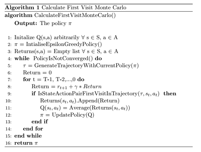
Let’s shortly talk through the pseudocode below.

At the beginning, we initialize all q-values with an arbitrary value. We furthermore use an epsilon greedy policy. Each q-value has a list of returns that are used to calculate the average. At the beginning we this list is empty.

The following part will be repeated until the algorithm converged.

We generate a trajectory \(\tau\) based on the current policy \(\pi\) and initialize the return of this trajectory to 0. Now, we start with the next to last state and update the return by the reward of this step and the returns from the next step. We start from behind, as this makes it easier to update the return.

If the state action value is the first visit from the start state, then we update the value. This means, we add this value to the list and calculate the average of them. If it is not the first visit, then nothing will be updated yet.

Now we continue with the previous state.

Summary

This post describes how we can use the First-Visit Monte Carlo to train our agent to solve the grid world. One advantage of this method is that the agent can directly learn from the experiences without the need of a model. Thus, we only require a way to sample from the environment, which is often not a problem. Especially, if we use a simulation.

A disadvantage is that the method requires a complete trajectory to learn from. Thus, in the next post, we will analyse a method that does not need the complete trajectory.